


We shall continue our analysis by further decompose the structural information into contributions from position and length scales. For simplicity, let us assume that we have a chemical system, characterised by concentrations ci(x, t) for the different molecules that are normalised at each position x,
![]() . (9)
. (9)
In order to be able to analyse
contributions from different length scales, we introduce a resolution dependent
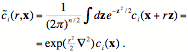
concentration ![]() , by convolution of the original one ci with a Gaussian,
, by convolution of the original one ci with a Gaussian,
 (10)
(10)
We will use the last expression
as the resolution operator, but when calculating ![]() , the first expression will be used. We assume that this
operation handles the boundary conditions so that in the limit of r ® ¥, i.e., complete loss of position information, the concentrations
equal the average concentrations in the system,
, the first expression will be used. We assume that this
operation handles the boundary conditions so that in the limit of r ® ¥, i.e., complete loss of position information, the concentrations
equal the average concentrations in the system,
![]() . (11)
. (11)
The derivation of a decomposition of the total information K into different contributions will now be slightly different from
the one in Chapter 6, since the distributions are now normalised in each
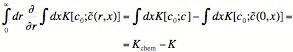
position (instead of over the system volume). Our starting point for decomposing the total information K,
 (12)
(12)
illustrates that the chemical information Kchem can be detected regardless of how bad the resolution
is. This is obvious, since complete loss of resolution results in average
concentrations in the system which determines the chemical information. This
means that the spatial information Kchem
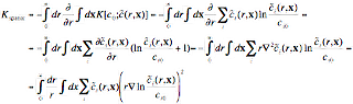
can be decomposed as follows
 (13)
(13)
In the last step a partial
integration is invoved, including an assumption of periodic (or non-flow)
boundary conditions. The equilibrium concentration ci0 in the last expressions could be removed (as it
disappears under the differential operation), but we keep it as it will serve a
purpose in later derivations. In the last expression we recognize a local
information density, k(r, x), which can be written in three
different forms, of which the last one will be used later,
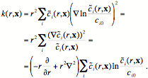 (14)
(14)
The information density k(r, x) can be integrated over space so
that we achieve the spatial information at a certain length scale,
![]() . (15)
. (15)
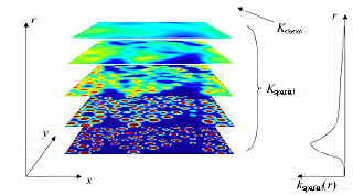
A schematic illustration of this decmposition is shown in the figure below,
illustrating a chemical patterns in a two-dimensional space with its variations
along the axis of resolution r.