PACE REPORT

We apply the formalism to the pattern formation of the “self-replicating spots” system (Gray and Scott, 1984; Pearson, 1993; Lee et al, 1993),

         U + 2V –> 3V,                                                                                     (31)

with the reaction-diffusion dynamics

                                                              (32)

We have introduced a very slow back reaction (k_back = 10^–5) in order to get the relationship between equilibrium concentrations of U and V defined by the reactions.

In the figure below, the dynamics is illustrated starting from an initial state (left) with a square of high concentration of V. As the system evolves four concentration peaks (spots) emerges from the square, and these spots reproduce by growing and splitting until the system is filled with spots (middle and right). In the process, spots may disappear, which leaves space for other spots to reproduce. In the lower part of the figure, the decomposition of the information in the pattern with respect to scale is plotted for the three snapshots above (at time 0, 1000, and 7000, respectively).

It is clear that the initial state has a longer characteristic length as detected by the information density. When the system produces the spots at the significantly shorter length scale, information is found both at the old length, now due to the size of the cluster (middle), and at the length scale of the spots. When the square distribution has been completely decomposed into spots, no information is left at the initial length scale.

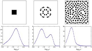
Figure 3. Top row: The concentration of the chemical V in the system at three times; t = 0, t = 1000, and t = 7000 steps. White corresponds to zero concentration, and black corresponds to a concentration of one half. Bottom row: The information density k(r, x), integrated over the system, as a function of the resolution r for the same time steps as above. The length of the system is 1, D_U = 2 D_V = 0.05, , k = 0.058. [Figure from (Lindgren et al 2004).]

In Fig. 4, we show the information density over the system for three different length scales after long time (upper part), and the information flow in scale, j_r, for the same state (lower part). At low resolution, or large r (right), the information density is low and captures structures of longer lengths, while at finer resolution, small r (left), the information density is large and reflects the pattern of spots. Note that each spot is seen as a circle in the information density picture, since the information is sensitive to gradients in the pattern. The information flow in scale, j_r, is close to homogenous for large r (right), but when information moves on to finer scales of resolution, the spatial flow j redistributes the flow so that a higher flow j_r is obtained at the concentration peaks. At finest resolution, r = 0, the information leaves the system as entropy production, which is mainly located to the concentration peaks where the chemical activity is high.

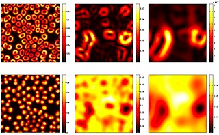
Figure 4. Top row: The information density k in the system at t = 10 000 steps, for three values of the resolution r; r = 0.01, r = 0.05, and r = 0.1. Bottom row: The information flow j_r(r, x, t). The length of the system is 1, D_U = 2, D_V = 0.05, , k = 0.058. [Figure from (Lindgren et al 2004).]

Simulations illustrating the process is also available:

--> Simulation of spots division

--> Simulation of information density at high resolution (cf. Fig. 4 top left)

--> Simulation of information density at lower resolution (cf. Fig. 4 top right)

--> Simulation of information flow at high resolution (cf. Fig. 4 lower left)

--> Simulation of information flow at lower resolution (cf. Fig. 4 lower right)